Time Series Analysis - ARIMA models - Model Estimation

V.I.2 Univariate Stochastic ARIMA Model Estimation

The estimation of ARMA parameters in practice is not straightforward. Though many computer algorithms and computer programs exist for ARMA estimation, care should be taken with respect to some important aspects. Since it is not our intention to go to far into the details of estimation algorithms, only some important pitfalls and problems are considered. These problems are especially interesting (important) for those who seek to apply the methodology in practice.

First, consider the formulation of the likelihood function. An ARIMA model contains three different kinds of parameters:

	the p AR-parameters;
	the q MA-parameters;
	and the variance of the error term.

This amount to a total of p + q + 1 parameters to be estimated (see also remark). These parameters are always estimated on using the stationary time series (c.q. a time series which is stationary with respect to it’s variance and mean): sometimes it is necessary to introduce an additional parameter m (a constant term) to be estimated such that the total amount of parameters to be estimated is p + q + 2.

(V.I.2-1)

likelihood function holds true.

The so-called log-likelihood function is

(V.I.2-2)

where SSR is the Sum of Squared Residuals

Box and Jenkins (1976) showed that the exact log-likelihood of an ARIMA model can be written as

(V.I.2-4)

Note the following definitions

(V.I.2-5)

and

(V.I.2-6)

Hence, using (V.I.2-4), it follows that

(V.I.2-7)

The backforecasting procedure is identical to the forecasting algorithm, except that the stationary time series is used in reversed order. Q' is identified by some criteria which ensure that the backforecasts have converged. This means that the backforecast should not be significantly different from the (zero) mean of e(t).

If backforecasting is not used (c.q. if the conditional likelihood criterion is used) the parameter estimates may deviate severely from the true parameters. Especially if the model contains MA parameters, exact likelihood estimation is necessary (see also the "truncation remainder").

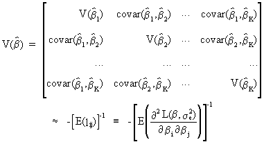
Note that the variance-covariance matrix of the estimated parameters is given by the inverse of the information matrix

(V.I.2-8)

which is derived from the likelihood function. Hence, not only the parameter estimation, but also the variances of the parameters are dependent on the use of the backforecasting procedure.

(V.I.2-9)

The large sample variance can be shown to be

(V.I.2-10)

Above that, Box and Jenkins prove that

and

are uncorrelated (for large samples). In fact, almost all estimation properties in time series analysis are large sample properties. The MLE estimates for ARIMA parameters are consistent, normally distributed, and asymptotically efficient.

It is possible that an estimation algorithm yields parameter values for an MA-process which lie outside the invertibility region. In such a case it is possible to find a SSR which is smaller than the true minimum.

The estimation process can be adequately performed by Marquardt's algorithm for nonlinear least squares as described in many references (BOX and JENKINS 1976), (MELARD 1984), (GARDNER, HARVEY, and PHILLIPS), etc...

Remark

Remark that it is assumed that there is no seasonality involved in the ARIMA process. In the case of seasonality, there would be p + P + q + Q + 1 parameters (P and Q being the seasonal counterparts of p and q respectively). Furthermore it is assumed that no constant term is required in the ARIMA process.