Plot the Time Series Data
This function is probably the most often used function. It
enables the user to show the time series by means of:
 | summarizing statistics | |
| a printed list of all observations (outliers are marked) | |
| a summary of outliers and extreme values | |
| a stem-and-leaf plot | |
| a chart of the time plot | |
Click the Time plot button in the RSF Toolbar:

This is the Time plot button

This is the RSF toolbar
Alternatively, you also may submit the command "timeplot"

Statistics
The summarizing statistics may look like this:
L:\ResaTest\Student\Airline.db by time


d = 0 D = 0 L = 1


Number of observations         = 144 (# observations lost = 0)

Median of Time Series          = 265,500000 * 1000 Units

2 Sided Trimmed Mean at 5%     = 275,606299 * 1000 Units

2 Sided Trimmed Mean at 10%    = 272,433628 * 1000 Units

2 Sided Trimmed Mean at 15%    = 270,515152 * 1000 Units

Mean of Time Series            = 280,298611 * 1000 Units

SE of Mean of Time Series      =  10,032087

T-STAT of Mean of Time Series  =  27,940208

SE of Time Series              = 119,966317

Mean without suspect values    = 280,298611 * 1000 Units

SE of Mean of Time Series      =  10,032087

T-STAT of Mean of Time Series  =  27,940208

SE without suspect values      = 119,966317

Minimum value of Time Series   = 104,000000 * 1000 Units

Maximum value of Time Series   = 622,000000 * 1000 Units

Minimum without suspect values = 104,000000 * 1000 Units

Maximum without suspect values = 622,000000 * 1000 Units
Observe how the mean of the time series is significantly
different from zero (the mean is 27.9 times larger than its Standard
Error). The time series under investigation has not been transformed
or differenced:
| d is the order of non-seasonal differencing. If d = 0, no
non-seasonal differencing is applied. | |
| D is the order of seasonal differencing. If D = 0, no seasonal
differencing is applied. | |
| L is the transformation parameter l:
if L = 1, no Box-Cox transformation is applied. | |
Values
The time series values are listed, and if case the time series is
stationary the outliers are marked (with a * symbol):
Observation  Value in Units * 1000


 1962/1      112,000000

 1962/2      118,000000

 1962/3      132,000000

 1962/4      129,000000

 1962/5      121,000000

 1962/6      135,000000

 1962/7      148,000000

 1962/8      148,000000

 1962/9      136,000000

 ...         ...
Since this time series is non-stationary, no outliers, nor
extreme values are marked. Summary of outliers and extreme values
If the time series is non-stationary, no outliers, nor extreme
values are reported.
Summary of extreme values:


Values > 2 S.E. at :


Values <-2 S.E. at :


Values > 3 S.E. at :


Values <-3 S.E. at :
Stem-and-Leaf Plot
The Stem-and-Leaf Plot provides you with quasi-visual impression
of the density of the time series:
  Explorative Data Analysis: Stem and Leaf Plot

     unit = 10

  1  2  represents 120


   23         1* 01111112222333334444444

   48          . 5566677777778888889999999

   69         2* 000011222233333333444

( 13)          . 5666677777789

   62         3* 000001111111133444444

   41          . 5555666667999

   28         4* 0000001112233

   15          . 66666779

    7         5* 0034

    3          . 5

    2         6* 02
Chart of the time series
The chart of the time series is displayed as a picture (jpg
format): 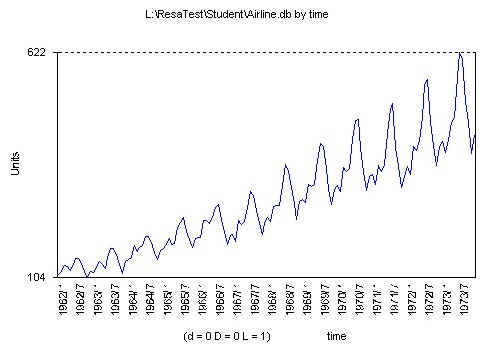
|