III.IV.2
Remedies to the multicollinearity problem
Let
us have a brief look at some possible solutions that may be used to
solve the harmful effects of the multicollinearity problem.
1.
drop spurious exogenous variables
Assume
we were interested in the estimation of the model

(III.IV.2-1)
where
G, I, H, L, and A are exogenous variables.
Suppose
that harmful multicollinearity would have been discovered between G,
I, and H and between L and A. Then we may chose one representative
of each group (e.g. G and L). All the other exogenous variables may
be dropped since they do not entail any information which is not
present in either G or L.
2.
principal components
As
we have seen before, X'X
can be diagonalized and written in terms of eigenvectors and
eigenvalues. Accordingly, the linear model can be written in terms
of its principal components (see (III.IV-4)).
The first principal component can intuitively be interpreted as the
summary of all exogenous variables by one column vector which
explains as much of X as
possible. The remaining information is entailed in the second
principal component and so on ... It is however important to note
that the principal components are orthogonal and therefore cannot be
multicollinear.
Suppose
we would have computed the principal components for our model of
(III.IV.2-1). Also assume that the principal components (PC) contain
(in descending order) 90%, 5%, 4%, ... of the total variance of the
exogenous variables. In such circumstances we would retain the first
three PC in our regression model since they account for 99% of the
variance of X.
When
having three PCs in a regression model, this means that there are
three important groups of variables (within the set of X)
which are explaining the endogenous variable. Cross correlations
between the exogenous variables and the PC should reveal which
variables may be associated with different factors (this is
necessary for interpretation purposes).
Now
suppose that this regression would result in only the first PC to be
significantly different from zero. In this case our model would
reduce to a simple regression. The only problem with this is that we
have no clue of how this model should be interpreted, since one PC
cannot directly be assigned to a specific exogenous variable (but
rather to a combination of all variables).
Therefore,
in such circumstances, it could be better to compute the PC for both
subgroups that we have detected before. We may present the X
matrix as follows
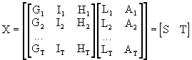
(III.IV.2-2)
and
compute the PC for S and T separately. This process will probably result in at least one
significant PC-parameter per subgroup in a multiple regression with
the endogenous, and therefore it is possible to interpret the model
easily. Note however that in this case there is no reason to assume
automatically that the first PC of S
and the first PC or T are
not multicollinear (since both PCs have been computed separately,
and since our detection of, and splitting the variables into two
subgroups, might have been wrong).
3.
ridge regression
The
estimator for ridge regression is
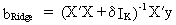
(III.IV.2-3)
where
delta is a small number which is to be added to the diagonal
elements of X'X. Be aware of the fact that there exists a sensitivity of the
parameters with respect to the ridge parameter delta (therefore
several values for delta might be attempted before deciding upon the
final ridge estimation results).
4.
first differences
The
first differences of a time series are defined by
(III.IV.2-4)
A
disadvantage of this differencing is obviously the loss of one
degree of freedom since the series becomes shorter. Also note that
this differencing is exclusively used with time series (and has
mostly no relevance with cross-section data).
The
relevance and interpretation will be comprehensively clarified in
chapter V (time series analysis).
The
only relevant thing to remember now, is that differencing alters the
time series so that it can be seen as the change
of the series. For instance the model

(III.IV.2-5)
illustrates
the effect of the change of Xt on the change of Yt.
When
a time series is differenced twice, it is not interpreted as the
absolute change but rather as the acceleration
of the series.
5).
ratio's and deflating series
It
is sometimes useful to use the ratio's of two (or more)
multicollinear series. In our example we could for instance redefine
the exogenous variables as
rgi
= G / I
rhi = H / I
rla = L / A
which
doesn't reduce the degrees of freedom, and maintains all variables
in the model. Though, care should be taken with respect to the
interpretation of the estimated parameters.
Another
common remedy to the multicollinearity problem is deflating time
series (mostly prices, or price indexes) by some time series
measuring e.g. consumption prices. Thus, in stead of working with
nominal quantities it is preferred to use real quantities.
6).
additional information and restrictions
Sometimes
economists have additional, or a priori information about the model.
This information could be in the form of knowledge about the true
value of some parameter, knowledge about an upper or lower bound for
parameters, or knowledge about dependencies between the sensitivity
parameters of different exogenous variables.
Such
information could be introduced into the model using Restricted
Least Squares (RLS) or Restricted
MLE (RMLE). For the moment, abstraction is made of Bayesian
methods where restrictions can be imposed stochastically in stead of
deterministically (see also chapter V). |